Visualizing Feature Maps using PyTorch
“What are feature maps ?”
Feature maps are nothing but the output, we get after applying a group of filters to the previous layer and we pass these feature maps to the next layer. Each layer applies some filters and generates feature maps. Filters are able to extract information like Edges, Texture, Patterns, Parts of Objects, and many more.
“Why we need to visualize Feature maps ?”
Normally it’s always a good habit to ask ‘why’ we are using this technique, before going to ‘how’ to implement this technique.
Deep Learning is good for many things like when our traditional approach fails deep learning may help, deep learning can easily adapt new scenerios, can you imagine trying to hand-craft rules for how ‘self-driving car’ should work No right, but deep learning can discover insights within large collections of data and figure out rules how ‘self-driving car’ should work.
With all this immense power of deep learning, still, the patterns learned by a deep learning model are typically uninterpretable by a human. We don’t know how my model predicting this target, what if my model predicts the wrong target. So I want to find out what features my model was focusing on or which filters my model applied.
Now here come in the picture ‘Feature maps’, feature maps help us to understand deep neural networks a little better.
“How we can visualize Feature maps ?”
pre-requisites:-
- The reader should have a basic understanding of Convolution Neural networks.
- We are using the PyTorch framework. PyTorch is an open-source machine learning library based on the Torch library, used for applications such as computer vision and natural language processing, primarily developed by Facebook’s AI Research lab. It is free and open-source software.
Import all the required libraries
import torch
import torch.nn as nn
import torchvision
from torchvision import models, transforms, utils
from torch.autograd import Variable
import numpy as np
import matplotlib.pyplot as plt
import scipy.misc
from PIL import Image
import json
%matplotlib inline
Define the image transformations
- Before passing the image to the model we make sure input images are of the same size
- CNN deals with the only tensor so we have to transform the input image to some tensor.
- One good practice is to normalize the dataset before passing it to the model.
transform = transforms.Compose([
    transforms.Resize((224, 224)),
    transforms.ToTensor(),
    transforms.Normalize(mean=0., std=1.)
])
Load Image
image = Image.open(str('dog.jpg'))
plt.imshow(image)
Load Model
Here we are using the Resnet18 model which is pretrained on the imagenet dataset, and it is only one line of code in pytorch to download and load the pre-trained resnet18 model. You can also write your own custom resnet architecture models. Here we are using a pre-trained one.
model = models.resnet18(pretrained=True)
print(model)
ResNet(
(conv1): Conv2d(3, 64, kernel_size=(7, 7), stride=(2, 2), padding=(3, 3), bias=False)
(bn1): BatchNorm2d(64, eps=1e-05, momentum=0.1, affine=True, track_running_stats=True)
(relu): ReLU(inplace=True)
(maxpool): MaxPool2d(kernel_size=3, stride=2, padding=1, dilation=1, ceil_mode=False)
(layer1): Sequential(
(0): BasicBlock(
(conv1): Conv2d(64, 64, kernel_size=(3, 3), stride=(1, 1), padding=(1, 1), bias=False)
(bn1): BatchNorm2d(64, eps=1e-05, momentum=0.1, affine=True, track_running_stats=True)
(relu): ReLU(inplace=True)
(conv2): Conv2d(64, 64, kernel_size=(3, 3), stride=(1, 1), padding=(1, 1), bias=False)
(bn2): BatchNorm2d(64, eps=1e-05, momentum=0.1, affine=True, track_running_stats=True)
)
(1): BasicBlock(
(conv1): Conv2d(64, 64, kernel_size=(3, 3), stride=(1, 1), padding=(1, 1), bias=False)
(bn1): BatchNorm2d(64, eps=1e-05, momentum=0.1, affine=True, track_running_stats=True)
(relu): ReLU(inplace=True)
(conv2): Conv2d(64, 64, kernel_size=(3, 3), stride=(1, 1), padding=(1, 1), bias=False)
(bn2): BatchNorm2d(64, eps=1e-05, momentum=0.1, affine=True, track_running_stats=True)
)
)
(layer2): Sequential(
(0): BasicBlock(
(conv1): Conv2d(64, 128, kernel_size=(3, 3), stride=(2, 2), padding=(1, 1), bias=False)
(bn1): BatchNorm2d(128, eps=1e-05, momentum=0.1, affine=True, track_running_stats=True)
(relu): ReLU(inplace=True)
(conv2): Conv2d(128, 128, kernel_size=(3, 3), stride=(1, 1), padding=(1, 1), bias=False)
(bn2): BatchNorm2d(128, eps=1e-05, momentum=0.1, affine=True, track_running_stats=True)
(downsample): Sequential(
(0): Conv2d(64, 128, kernel_size=(1, 1), stride=(2, 2), bias=False)
(1): BatchNorm2d(128, eps=1e-05, momentum=0.1, affine=True, track_running_stats=True)
)
)
(1): BasicBlock(
(conv1): Conv2d(128, 128, kernel_size=(3, 3), stride=(1, 1), padding=(1, 1), bias=False)
(bn1): BatchNorm2d(128, eps=1e-05, momentum=0.1, affine=True, track_running_stats=True)
(relu): ReLU(inplace=True)
(conv2): Conv2d(128, 128, kernel_size=(3, 3), stride=(1, 1), padding=(1, 1), bias=False)
(bn2): BatchNorm2d(128, eps=1e-05, momentum=0.1, affine=True, track_running_stats=True)
)
)
(layer3): Sequential(
(0): BasicBlock(
(conv1): Conv2d(128, 256, kernel_size=(3, 3), stride=(2, 2), padding=(1, 1), bias=False)
(bn1): BatchNorm2d(256, eps=1e-05, momentum=0.1, affine=True, track_running_stats=True)
(relu): ReLU(inplace=True)
(conv2): Conv2d(256, 256, kernel_size=(3, 3), stride=(1, 1), padding=(1, 1), bias=False)
(bn2): BatchNorm2d(256, eps=1e-05, momentum=0.1, affine=True, track_running_stats=True)
(downsample): Sequential(
(0): Conv2d(128, 256, kernel_size=(1, 1), stride=(2, 2), bias=False)
(1): BatchNorm2d(256, eps=1e-05, momentum=0.1, affine=True, track_running_stats=True)
)
)
(1): BasicBlock(
(conv1): Conv2d(256, 256, kernel_size=(3, 3), stride=(1, 1), padding=(1, 1), bias=False)
(bn1): BatchNorm2d(256, eps=1e-05, momentum=0.1, affine=True, track_running_stats=True)
(relu): ReLU(inplace=True)
(conv2): Conv2d(256, 256, kernel_size=(3, 3), stride=(1, 1), padding=(1, 1), bias=False)
(bn2): BatchNorm2d(256, eps=1e-05, momentum=0.1, affine=True, track_running_stats=True)
)
)
(layer4): Sequential(
(0): BasicBlock(
(conv1): Conv2d(256, 512, kernel_size=(3, 3), stride=(2, 2), padding=(1, 1), bias=False)
(bn1): BatchNorm2d(512, eps=1e-05, momentum=0.1, affine=True, track_running_stats=True)
(relu): ReLU(inplace=True)
(conv2): Conv2d(512, 512, kernel_size=(3, 3), stride=(1, 1), padding=(1, 1), bias=False)
(bn2): BatchNorm2d(512, eps=1e-05, momentum=0.1, affine=True, track_running_stats=True)
(downsample): Sequential(
(0): Conv2d(256, 512, kernel_size=(1, 1), stride=(2, 2), bias=False)
(1): BatchNorm2d(512, eps=1e-05, momentum=0.1, affine=True, track_running_stats=True)
)
)
(1): BasicBlock(
(conv1): Conv2d(512, 512, kernel_size=(3, 3), stride=(1, 1), padding=(1, 1), bias=False)
(bn1): BatchNorm2d(512, eps=1e-05, momentum=0.1, affine=True, track_running_stats=True)
(relu): ReLU(inplace=True)
(conv2): Conv2d(512, 512, kernel_size=(3, 3), stride=(1, 1), padding=(1, 1), bias=False)
(bn2): BatchNorm2d(512, eps=1e-05, momentum=0.1, affine=True, track_running_stats=True)
)
)
(avgpool): AdaptiveAvgPool2d(output_size=(1, 1))
(fc): Linear(in_features=512, out_features=1000, bias=True)
)
As you can see above resnet architecture we have a bunch of Conv2d, BatchNorm2d, and ReLU layers. But I want to check only feature maps after Conv2d because this the layer where actual filters were applied. So let’s extract the Conv2d layers and store them into a list also extract corresponding weights and store them in the list as well.
# we will save the conv layer weights in this list
model_weights =[]
#we will save the 49 conv layers in this list
conv_layers = []# get all the model children as list
model_children = list(model.children())#counter to keep count of the conv layers
counter = 0#append all the conv layers and their respective wights to the list
for i in range(len(model_children)):
    if type(model_children[i]) == nn.Conv2d:
        counter+=1
        model_weights.append(model_children[i].weight)
        conv_layers.append(model_children[i])
    elif type(model_children[i]) == nn.Sequential:
        for j in range(len(model_children[i])):
            for child in model_children[i][j].children():
                if type(child) == nn.Conv2d:
                    counter+=1
                    model_weights.append(child.weight)
                    conv_layers.append(child)
print(f"Total convolution layers: {counter}")
print("conv_layers")
Total convolution layers: 17
[Conv2d(3, 64, kernel_size=(7, 7), stride=(2, 2), padding=(3, 3), bias=False),
Conv2d(64, 64, kernel_size=(3, 3), stride=(1, 1), padding=(1, 1), bias=False),
Conv2d(64, 64, kernel_size=(3, 3), stride=(1, 1), padding=(1, 1), bias=False),
Conv2d(64, 64, kernel_size=(3, 3), stride=(1, 1), padding=(1, 1), bias=False),
Conv2d(64, 64, kernel_size=(3, 3), stride=(1, 1), padding=(1, 1), bias=False),
Conv2d(64, 128, kernel_size=(3, 3), stride=(2, 2), padding=(1, 1), bias=False),
Conv2d(128, 128, kernel_size=(3, 3), stride=(1, 1), padding=(1, 1), bias=False),
Conv2d(128, 128, kernel_size=(3, 3), stride=(1, 1), padding=(1, 1), bias=False),
Conv2d(128, 128, kernel_size=(3, 3), stride=(1, 1), padding=(1, 1), bias=False),
Conv2d(128, 256, kernel_size=(3, 3), stride=(2, 2), padding=(1, 1), bias=False),
Conv2d(256, 256, kernel_size=(3, 3), stride=(1, 1), padding=(1, 1), bias=False),
Conv2d(256, 256, kernel_size=(3, 3), stride=(1, 1), padding=(1, 1), bias=False),
Conv2d(256, 256, kernel_size=(3, 3), stride=(1, 1), padding=(1, 1), bias=False),
Conv2d(256, 512, kernel_size=(3, 3), stride=(2, 2), padding=(1, 1), bias=False),
Conv2d(512, 512, kernel_size=(3, 3), stride=(1, 1), padding=(1, 1), bias=False),
Conv2d(512, 512, kernel_size=(3, 3), stride=(1, 1), padding=(1, 1), bias=False),
Conv2d(512, 512, kernel_size=(3, 3), stride=(1, 1), padding=(1, 1), bias=False)]
Check for GPU
device = torch.device(‘cuda’ if torch.cuda.is_available() else ‘cpu’)
model = model.to(device)
Apply transformation on the image, Add the batch size, and load on GPU
image = transform(image)
print(f"Image shape before: {image.shape}")
image = image.unsqueeze(0)
print(f"Image shape after: {image.shape}")
image = image.to(device)
Generate feature maps
Process image to every layer and append output and name of the layer to outputs[] and names[] lists
outputs = []
names = []
for layer in conv_layers[0:]:
    image = layer(image)
    outputs.append(image)
    names.append(str(layer))
print(len(outputs))#print feature_maps
for feature_map in outputs:
    print(feature_map.shape)
torch.Size([1, 64, 112, 112])
torch.Size([1, 64, 112, 112])
torch.Size([1, 64, 112, 112])
torch.Size([1, 64, 112, 112])
torch.Size([1, 64, 112, 112])
torch.Size([1, 128, 56, 56])
torch.Size([1, 128, 56, 56])
torch.Size([1, 128, 56, 56])
torch.Size([1, 128, 56, 56])
torch.Size([1, 256, 28, 28])
torch.Size([1, 256, 28, 28])
torch.Size([1, 256, 28, 28])
torch.Size([1, 256, 28, 28])
torch.Size([1, 512, 14, 14])
torch.Size([1, 512, 14, 14])
torch.Size([1, 512, 14, 14])
torch.Size([1, 512, 14, 14])
Now convert 3D tensor to 2D, Sum the same element of every channel
processed = []
for feature_map in outputs:
    feature_map = feature_map.squeeze(0)
    gray_scale = torch.sum(feature_map,0)
    gray_scale = gray_scale / feature_map.shape[0]
    processed.append(gray_scale.data.cpu().numpy())for fm in processed:
    print(fm.shape)
(112, 112)
(112, 112)
(112, 112)
(112, 112)
(112, 112)
(56, 56)
(56, 56)
(56, 56)
(56, 56)
(28, 28)
(28, 28)
(28, 28)
(28, 28)
(14, 14)
(14, 14)
(14, 14)
(14, 14)
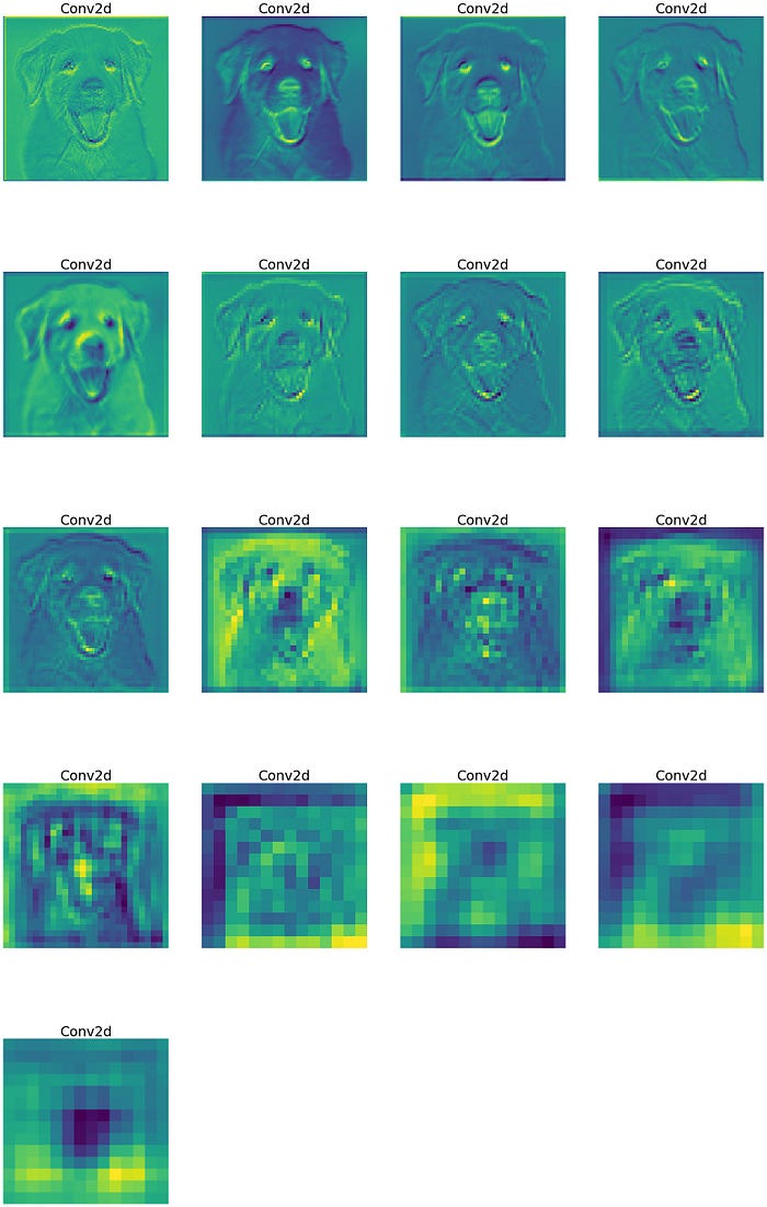
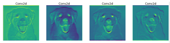
Plotting feature maps and save
fig = plt.figure(figsize=(30, 50))
for i in range(len(processed)):
    a = fig.add_subplot(5, 4, i+1)
    imgplot = plt.imshow(processed[i])
    a.axis("off")
    a.set_title(names[i].split('(')[0], fontsize=30)
plt.savefig(str('feature_maps.jpg'), bbox_inches='tight')